Comprehensive overview of learning rate schedulers in Machine Learning
The learning rate is a crucial hyperparameter that directly affects the future model’s performance. It represents the size of your model’s weight updates in search of the global minimal loss value.
In short, learning rate schedulers are algorithms that allow you to control your model’s learning rate according to some pre-set schedule or based on performance improvements.
On this page, we will observe:
- What are gradient descent and learning rate in Machine Learning;
- What is the idea behind learning rate schedulers, and how do they work;
- How to play with schedulers in Hasty.
Let’s jump in.
Learning rate schedulers explained
Gradient descent
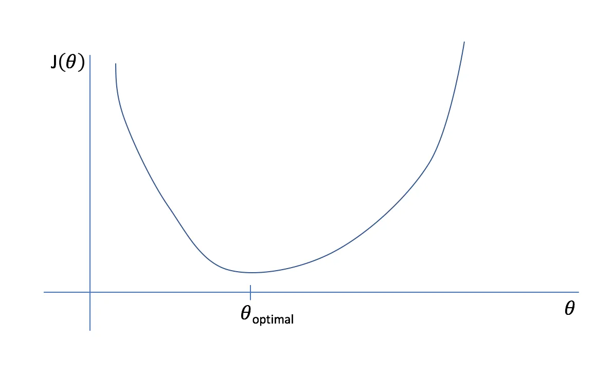
Gradient descent is an optimization technique that helps researchers detect the most optimal model weight values on training.
An effective way to assess the model’s performance on training is to set the cost function, also called a loss function. In the Data Science field, such a function focuses on punishing a model for making errors by assigning some cost to mistakes. Thus, in theory, we can find out the position of our model on the loss function curve for each set of parameters. The weights that result in the minimal loss function lead to the best model performance.
Source
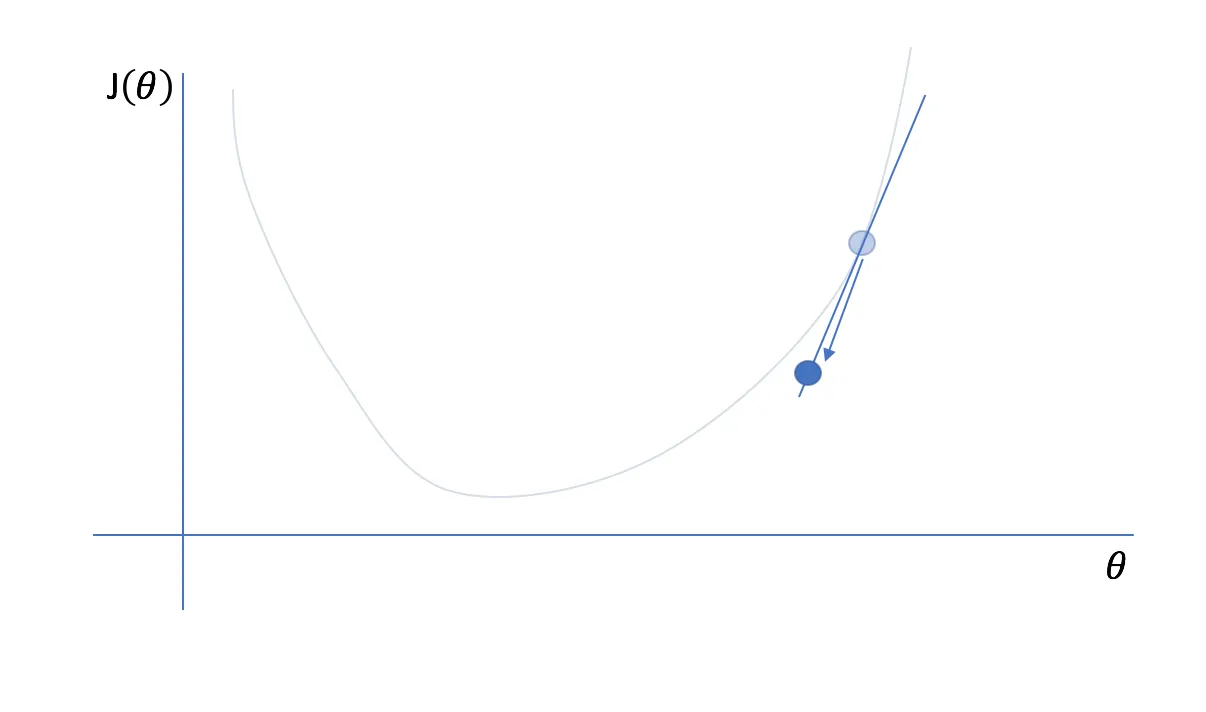
In the real world, we usually can not afford to check the model’s loss function for every possible set of parameters since the computation costs would be too high. Therefore, starting with some random guess and then refining it in iterations makes sense. The algorithm is as follows:
- Calculate the loss function for the initial guess (usually random parameter values).
- Slightly change the parameters and see if the loss function value has increased or decreased.
- Move towards the direction where the loss function decreases.
- Repeat steps 2 and 3 until one of the stopping criteria is met:
- The limit of iterations is exceeded;
- The step size (the update) is smaller than the defined minimum, meaning that the loss value practically does not change.
Source
Learning rate
The learning rate is a hyperparameter that determines the size of the weights update your model makes at each step.
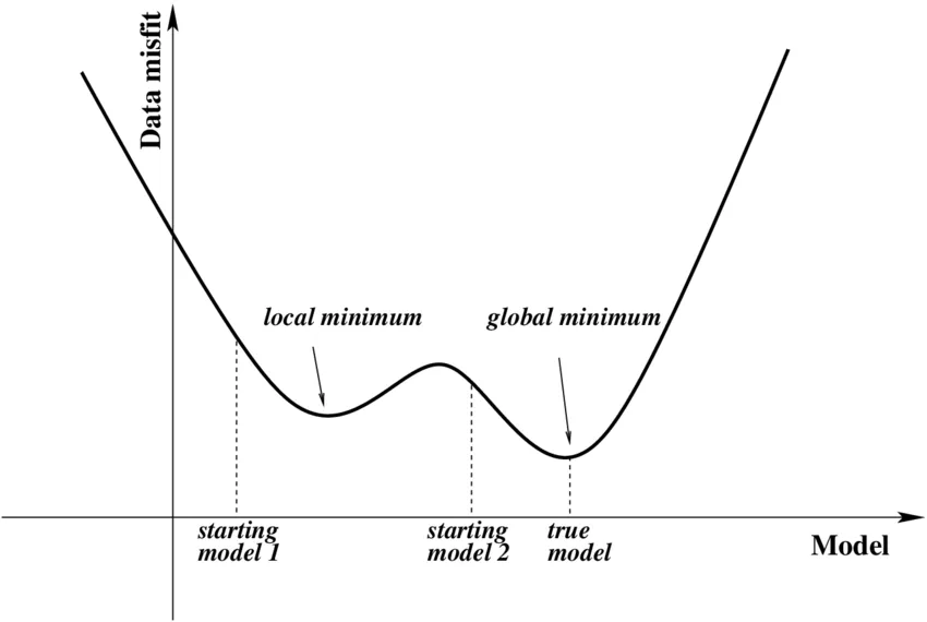
Choosing the optimal learning rate can be problematic. One of the challenges that may arise is the so-called local minimum problem.
Source
When your model starts moving towards the local minimum, the slope of the change will approach zero. If the update size is small, your model might stop running new iterations as it thinks the global minimum has been reached and there are no better points to look for. Thus, the model never converges to the global minimum and stays at the sub-optimal point.
To avoid ending up with too small step sizes and getting stuck in the local minimum, it might seem reasonable to set a high learning rate. However, a more significant learning rate could lead to the model passing by the optimal point without noticing it. Moreover, drastic updates might result in inadequate training, as seen in the picture below.
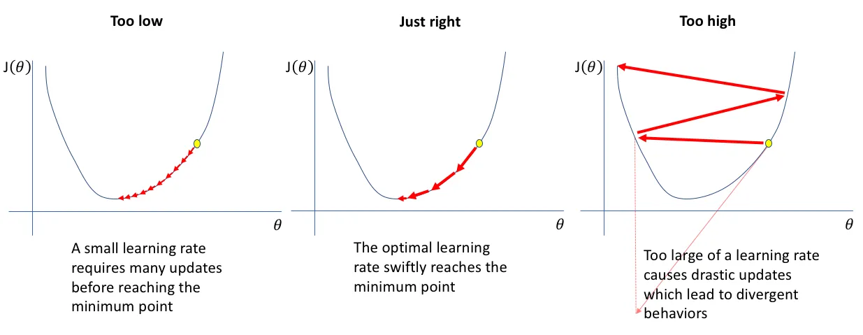
To sum up:
- A higher learning rate speeds up the model convergence but might miss the most optimal point;
- A lower learning rate is more sensitive to the loss function changes but may consume too much computational power and get stuck in local minima.
To address the issue, learning rate schedulers come into play.
Schedulers
The learning rate schedulers are algorithms that allow you to control your model’s learning rate according to some schedule.
For instance, you might want to start with a more significant learning rate and then slowly decay it as the loss value approaches the global minimum, or you might increase and decrease the learning rate in cycles.
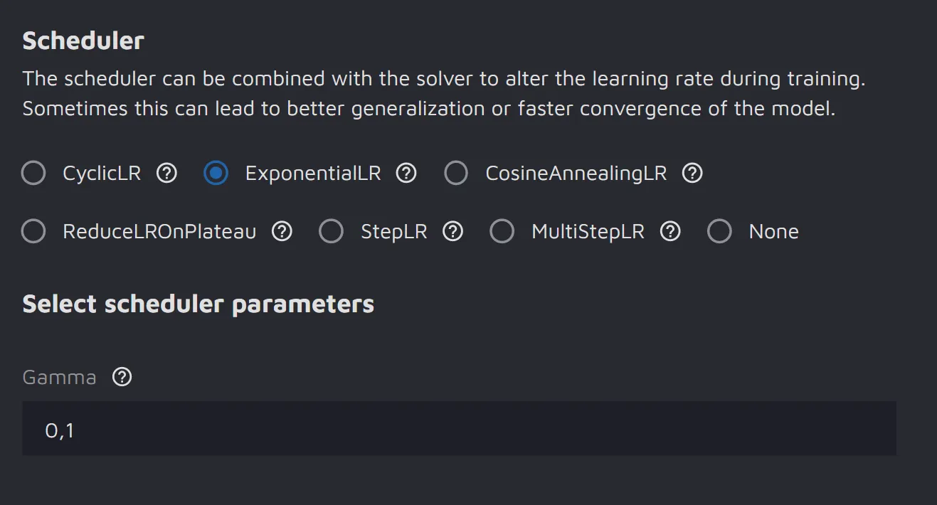
There are many types of schedulers. Below are the learning rate schedulers that Hasty offers:
- ExponentialLR - every epoch/evaluation period, it divides the learning rate by the same factor named gamma;
- CyclicLR - varies the learning rate between the minimal and maximal thresholds in cycles;
- StepLR - decays the learning rate by gamma every N epochs/evaluation periods;
- MultiStepLR - decays the learning rate of each parameter group by gamma once the number of epochs reaches one of the milestones;
- ReduceLROnPlateau - decreases the learning rate when the specified metric stops improving for longer than the patience number allows;
- CosineAnnealingLR - starts with a very high learning rate value and then aggressively decreases it to a value near 0 before increasing the learning rate again.
How to use schedulers in Hasty
1. Open the Project Dashboard;
2. Click on the Model Playground section;
3. Select the split and create an experiment;
4. In the experiment parameters, open the Solver & scheduler section;

5. Select the Solver (optimizer) model and set the Base learning rate;
6. Choose the Scheduler and set the corresponding parameters;
7. Start the experiment and enjoy the results :)