Convolutional layer
When it comes to the fundamental principles one should understand to work in a Computer Vision field, the excellent place to start is through grinding the convolution concept. On this page, we will:
Check out the convolution definition in Machine Learning (ML);
Understand how to apply convolutions to RGB images;
See the differences between 1D, 2D, and 3D convolutions;
Identify why convolution is essential for Computer Vision;
Calculate 2D and RGB convolutions on simple examples;
Check out the code implementation of 1D, 2D, and 3D convolutions in PyTorch.
Let’s jump in.
What is a Machine Learning convolution?
Machine Learning convolution definition is rather simple but might require some time to process and fully understand.
To define the term, Machine Learning convolution is an application operation between two data matrices - the first, smaller one, is called a convolution kernel K, whereas the second one, M is bigger and used as input data to which the convolution is applied.
The basic convolution scenario is called 2D convolution. The general algorithm of the Machine Learning 2D convolution is as follows:
You have two matrices - a smaller K and a larger input matrix, M. Both of them are two-dimensional;
You place K in the top left corner of M;
You perform an element-wise multiplication between the K and the corresponding elements of M;
The multiplication results are summed up, and the output value is placed in the corresponding position in the output matrix O;
You repeat steps 3 and 4 while your kernel is “sliding” over M. “Sliding” means that you move the kernel to the right (or back to the left matrix border and down if there is no room on the right) on some fixed number of pixels until K reaches the bottom right corner of M.

M is the light blue matrix
K is the dark blue matrix
O is the white matrix
The sliding step is 1
Source
How to apply 2D convolution to an RGB image?
The 2D convolution concept can be applied to colored images with slight modifications. A colored image has 3 channels - Red, Green, and Blue. Each of these channels is a 2D matrix.

Source
When applying convolution to RGB images, the most significant difference is in the terminology. As mentioned above, for 2D convolution, the kernel and filter terms are interchangeable. However, when convolution expands by adding another dimension or input channel, the filter becomes a collection of kernels. In a filter, there is a kernel for each input channel, and each kernel is unique.
For example, for a 3-channel RGB input, the filter will consist of 3 kernels corresponding to R, G, and B channels.
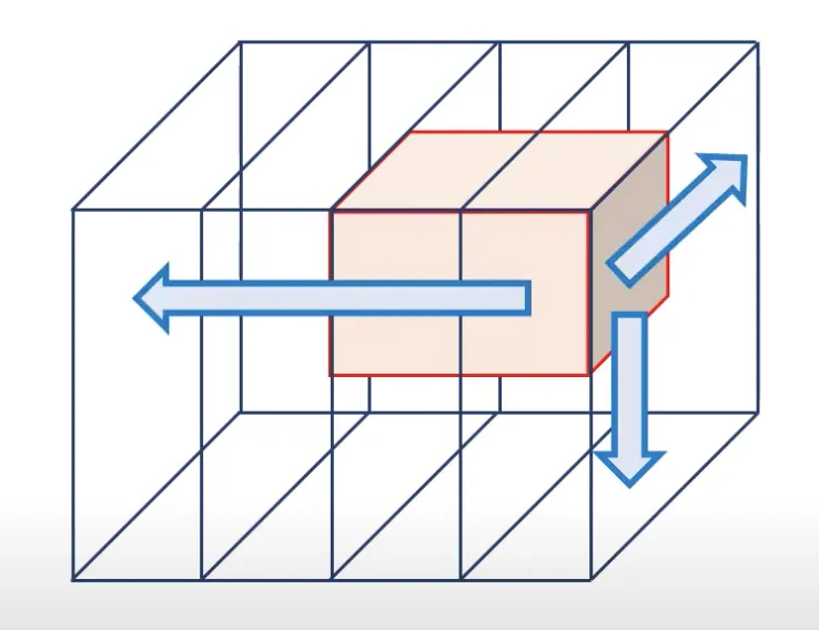
The general algorithm of the Machine Learning 3D and multi-channel convolution is as follows:
You have a filter F and a larger multi-channel input, M;
You place each kernel from F in the top left corner of the corresponding layer of M;
You perform a standard 2D convolution procedure until each kernel from F reaches the bottom right corner of the corresponding layer of M;
As a result, you get N output matrices o, where N is the number of channels;
You sum N matrices o to get the general cross-channel output matrix O;
(optional) You might add a linear bias to O, but it should be the same value for a whole filter.

Source

Light red, green, and blue matrices are o
O is the yellow matrix
Source

Convolution process finishes with the addition of a linear bias
O is the yellow matrix
Linear bias is the orange block
Light orange matrix is the final output
Source
1D convolution Vs. 2D convolution Vs. 3D convolution
2D convolution is a strong basis but can only cover some potential needs and cases. Therefore, to fill the gaps, there are 1D and 3D convolutions.
From a mathematical standpoint, they are similar to 2D convolution as they stay a linear matrix transformation. The critical difference is the number of dimensions the filter can operate with.
For 2D convolution, the filter slides from top to bottom and left to right. Hence, it is called 2D convolution.

Source
3D convolution adds another dimension. An excellent example of a case that might require 3D convolution is a video. For example, you might have a color video containing 4 frames as an input. Therefore, you will also need to move the filter along the time axis.
Thus, as well as moving from top to bottom and from left to right, the filter also moves from the beginning to the end of a videotape. The filter moves in 3 directions, so such a convolution is a 3D one.
Source
However, if the filter size for the time dimension is equal to 4 (as we had 4 frames as an input), such a case would be considered a 2D convolution one.

Source
Another potential case is 1D convolution. For such a scenario, a filter should be the same size as the input channel and have only one direction to slide along.

Source
As you can see, 1D, 2D, and 3D convolutions vary by the number of directions the filter can slide along when performing linear matrix transformations.
Real-life convolutional layer use case
As you might know, any visual data can be viewed as a matrix where each cell represents a specific pixel. The convolution concept operates with matrices. This is what makes convolution a perfect fit for Computer Vision tasks.
The ultimate goal of convolution is to extract valuable features from the visual data that can be used for further interpretation and analysis via other technical approaches, such as a multilayer perceptron (MLP).
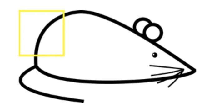
Let’s check out the convolution operation on a high level. Imagine having a black-and-white image of a mouse.

Source
Each filter can be viewed as a feature identifier. The features are some simple characteristics all the images have in common such as straight borders, simple colors, various curves, etc. Our first filter will be a 7 x 7 curve detector.

Source
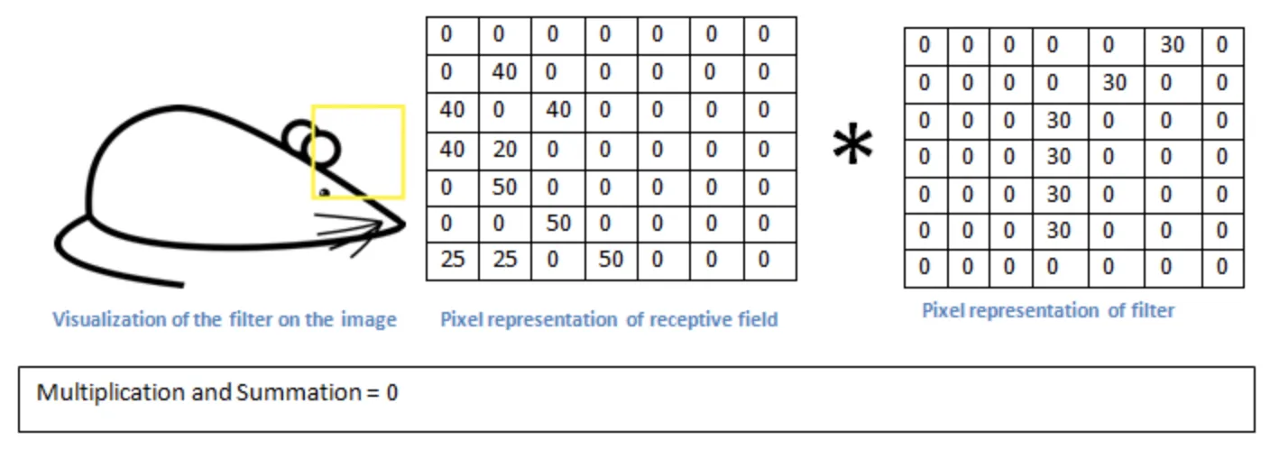
Let’s apply the filter to the upper-left corner of the original image, perform the convolution operation and calculate the output value.
Source

Source
As you can see, the output value is a large number. This happens because the upper-left corner of the original image had a curve similar to the one in a filter. Therefore, the network will know that the upper-left corner of the picture has a curve convex upwards to the left.
However, if you apply the same filter to the upper-right corner of the image, you will see a completely different result.
Source
As you can see, the value is significantly lower. This happens because there is nothing similar to the curve filter in the upper-right corner of the image.
The output of any convolutional layer is a feature map in the form of a matrix. In our case (with only one curve filter), the feature map will have high values in the cells that correspond to the areas of the original image where a specific curve is more likely to be present.
So, in the upper left corner, the value of the feature map would be 6600. This high value indicates that the filter has seen some shape similar to the filter's curve. In the upper right corner, the value of the feature map will be 0 because there was no similar curve in this area.
Please remember that in this example, we had only one filter. In a real-life scenario, there may be many filters, making feature maps less interpretable. However, more filters lead to a greater depth of the feature map and more valuable information about the initial image. This will greatly help MLPs to analyze the convolutions' output further.

Source
Machine Learning convolution calculation example
Let’s check out some practical examples of calculating convolutions.
2D convolution calculation example
Imagine having a 4x4 input matrix and a 2x2 kernel. The kernel “sliding” step will be 1, so we will move by one cell at a time.
1 | 2 | 3 | 4 |
5 | 6 | 7 | 8 |
9 | 10 | 11 | 12 |
13 | 14 | 15 | 16 |
1 | 2 |
3 | 4 |
Let’s start.
1 * 1 = 1 | 2 * 2 = 4 | 3 | 4 |
5 * 3 = 15 | 6 * 4 = 24 | 7 | 8 |
9 | 10 | 11 | 12 |
13 | 14 | 15 | 16 |
1 + 4 + 15 + 24 = 44 - this will be the value for the top left cell of the output matrix.
1 | 2 * 1 = 2 | 3 * 2 = 6 | 4 |
5 | 6 * 3 = 18 | 7 * 4 = 32 | 8 |
9 | 10 | 11 | 12 |
13 | 14 | 15 | 16 |
2 + 6 + 18 + 32 = 58 - this will be the value for the second cell of the top row of the output matrix.
1 | 2 | 3 * 1 = 3 | 4 * 2 = 8 |
5 | 6 | 7 * 3 = 21 | 8 * 4 = 32 |
9 | 10 | 11 | 12 |
13 | 14 | 15 | 16 |
3 + 8 + 21 + 32 = 64 - this will be the value for the third cell of the top row of the output matrix.
1 | 2 | 3 | 4 |
5 * 1 = 5 | 6 * 2 = 12 | 7 | 8 |
9 * 3 = 27 | 10 * 4 = 40 | 11 | 12 |
13 | 14 | 15 | 16 |
5 + 12 + 27 + 40 = 84 - this will be the value for the first cell of the second row of the output matrix.
At this point, the output matrix looks as follows.
44 | 58 | 64 |
84 |
|
|
|
|
|
Please continue filling it in for a slight training and a better understanding of the convolution process.
RGB image 2D convolution calculation example
Overall, RGB image convolution calculation is not that different from the previous example. The task is expanded as you need to perform 2D convolution several times instead of one and perform additional steps to get the final value.
Perform 2D convolution for each corresponding input channel and kernel;
Summarize the output values;
(optional) Add bias;
Place the final value in the corresponding cell of the output matrix.

Source
Convolutional layer in Python
All the convolution types are widely supported by all the modern Deep Learning frameworks. As the name suggests, convolutional layers are the basis of Convolutional Neural Networks. Therefore, all the options provided by TensorFlow, Keras, MxNet, PyTorch, etc., are valid, valuable, and worth your attention if you prefer a specific framework.