Focal loss
We have already discussed Cross-Entropy Loss and Binary Cross-Entropy Loss for the classification problem. Focal loss is an extension of these losses with new parameters that give more weight to "hard" samples and less weight to "easy" samples. We shall discuss more thoroughly what the hard and easy samples refer to.
Class Imbalance might happen if information relayed to one class in a dataset over-represents the rest of the classes. Training a network in such an imbalanced data set might cause the network to be more biased towards learning more of the data-dominated class.
This type of imbalance might happen in two ways. First, it can happen between the classes of the foreground image, for example having 20 times more pictures of dogs than other animals in an animal detection problem. Second, there might be more background anchors than foreground anchors.
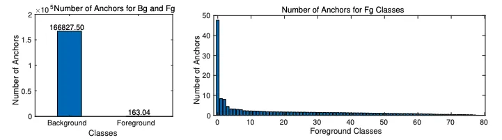
Let us look at the first figure. Since there is almost a thousand times more background than the foreground images, more background images are the easy samples because they are easier to detect and more foreground images are the hard samples. Therefore, the loss in background classification is considerably lower than the foreground classification for a single image. But, if we sum all the errors, then the background loss can overwhelm the foreground loss despite having fewer individual losses.
To counteract this problem posed by class imbalance, we introduce Focal Loss.
Intuition
We use a scaling factor along with the Cross-Entropy Loss in order to down-weight the easy samples and give more weight to the hard samples. In other words, we modulate the cross-entropy such that the training process can focus on the hard negative samples.
Focal Loss in Model Playground
Alpha
This term is the in the following formula for Focal Loss. This alpha offsets the class imbalance of the number of examples. This alpha is set inversely proportional to the number of examples for a particular class or is learned through cross-validation.
Gamma
This term is used to focus on the hard examples. The hard and easy examples are defined by the probability of the correct classification, . If is low, then we are dealing with a hard sample. In this case, the modulating factor, remains near 1 and is unaffected. If is high then the modulating factor vanishes to 0. This gives lower weight to the easy samples.