SGD

Deep learning optimizer literature starts with Gradient Descent and the Stochastic Gradient Descent (SGD) is one very widely used version of it. The gradients are not calculated for the loss functions over all data points but over a randomly selected sub-sample. This is why it is also called mini-batch gradient descent sometimes.

Most relevant hyper-parameters of SGD:

• Base learning rate
• Momentum
• Dampening
• Weight decay

Intuition

Gradient Descent

The goal of each solver is to find the loss function's minimum. However, this cannot be done by just setting the derivative to 0 (as you learned to do in calculus I) because there is no closed-form solution. This is because the loss landscape of neural networks is highly non-convex and riddled with saddle points.

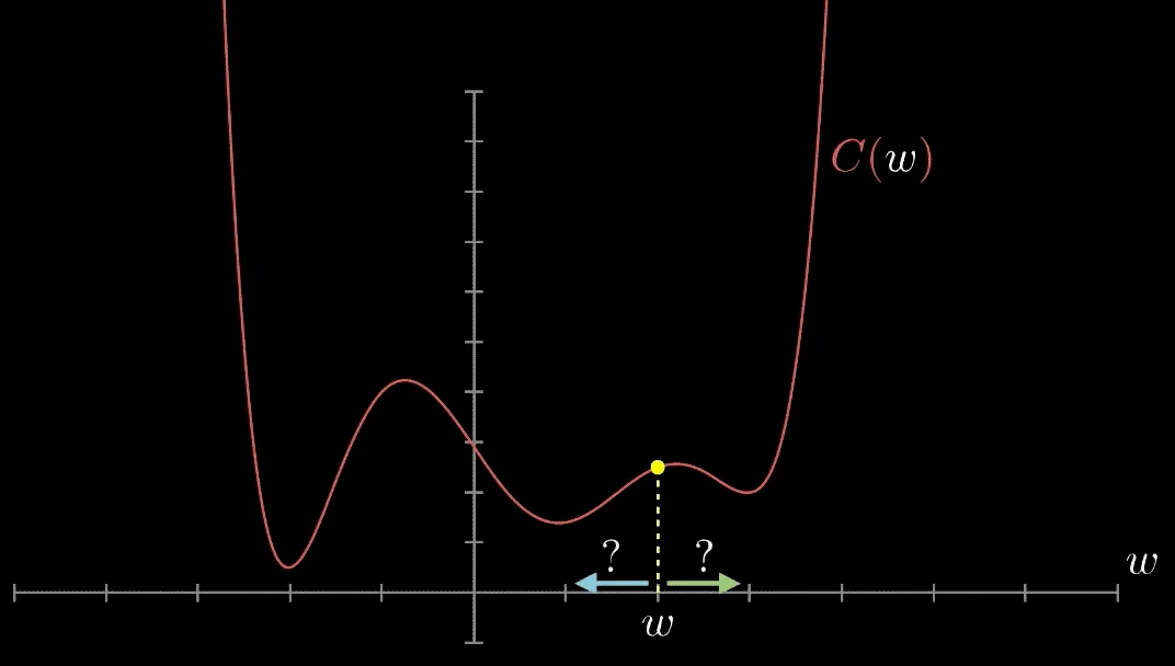
Have you met Gradient Descent? Gradient Descent is an algorithm that finds local minima. It calculates the gradient of a given point on a loss function. If the gradient is negative, it updates the weights moving to a point in the direction of the gradient; if it's positive to a point in the opposite direction. This is repeated until the algorithm converges. Then, we have found a local minimum—or are at least are very close to it.

In the vanilla form, the only parameter to know is the base learning rate.

Stochastic Gradient Descent (SGD)

SGD is a more computationally efficient form of Gradient Descent.

SGD only estimates the gradient for the loss from a small sub sample of data point only, enabling it to run much faster through the iterations. Theoretically speaking, the loss function is not as well minimized as with BGD. However, in practice, the close approximation that you get in SGD for the parameter values can be close enough in many cases. Also, the stochasticity is a form of regularization, so the networks usually generalize better.

Code implementation

PyTorch

# importing the library
import torch
import torch.nn as nn

x = torch.randn(10, 3)
y = torch.randn(10, 2)

# Build a fully connected layer.
linear = nn.Linear(3, 2)

# Build MSE loss function and optimizer.
criterion = nn.MSELoss()

# Optimization method uses random gradient descent, the learning rate is 0.01 and the momentum 0.9
optimizer = torch.optim.SGD(linear.parameters(), lr=0.01, momentum=0.9)

# Forward pass.
pred = linear(x)

# Compute loss.
loss = criterion(pred, y)
print('loss:', loss.item())

optimizer.step()

TensorFlow

# importing the library
import tensorflow as tf

opt = tf.keras.optimizers.SGD(learning_rate=0.1, momentum=0.9)
var = tf.Variable(1.0)
val0 = var.value()
loss = lambda: (var ** 2)/2.0         # d(loss)/d(var1) = var1

# First step is `- learning_rate * grad`
step_count = opt.minimize(loss, [var]).numpy()
val1 = var.value()
print((val0 - val1).numpy())

# On later steps, step-size increases because of momentum
step_count = opt.minimize(loss, [var]).numpy()
val2 = var.value()
print((val1 - val2).numpy())

Further resources

• Base learning rate
• Dampening
• Momentum
• Weight decay
• Adam
• AdamW
• Image Source