mean Average Precision (mAP)
If you have ever worked on an Object Detection, Instance Segmentation, or Semantic Segmentation tasks, you might have heard of the popular mean Average Precision (mAP) Machine Learning (ML) metric. On this page, we will:
Сover the logic behind the metric;
Check out the mean Average Precision formula;
Find out how to interpret the metric’s value;
Present a simple mean Average Precision calculation example;
And see how to work with mAP using Python.
Let’s jump in.
What is mean Average Precision?
To define the term, mean Average Precision (or mAP) is a Machine Learning metric designed to evaluate the Object Detection algorithms. To clarify, nowadays, you can use mAP to evaluate Instance and Semantic Segmentation models as well. Still, we will not talk much about these use cases on this page as we will focus on mean Average Precision for Object Detection tasks.
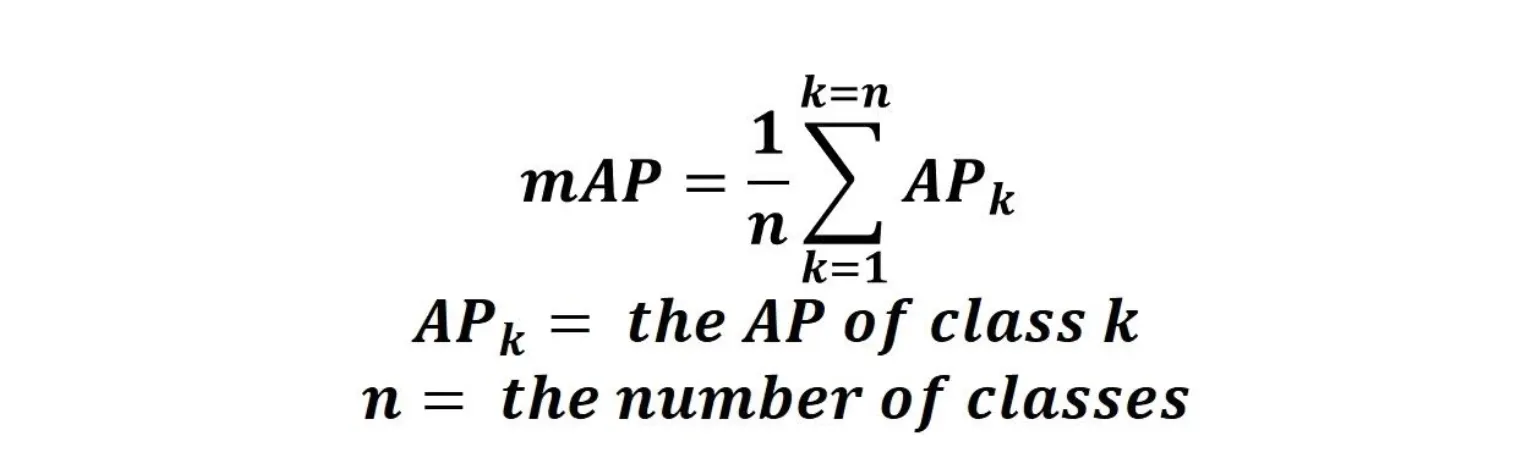
mean Average Precision formula
From the mathematical standpoint, computing mAP requires summing up the Average Precision scores across all the classes and dividing the result by the total number of classes.
Source
Still, it is not that easy. In Object Detection-related papers, you can face such abbreviations as [email protected] or [email protected]. In short, this notation depicts the IoU threshold used to calculate mAP. Let’s check out how it works.
Object 1 | 0.95 | Correct Prediction | Correct Prediction | Correct Prediction |
Object 2 | 0.9 | Incorrect Prediction | Correct Prediction | Correct Prediction |
Object 3 | 0.85 | Incorrect Prediction | Correct Prediction | Correct Prediction |
Object 4 | 0.8 | Incorrect Prediction | Correct Prediction | Correct Prediction |
Object 5 | 0.7 | Incorrect Prediction | Incorrect Prediction | Correct Prediction |
Object 6 | 0.4 | Incorrect Prediction | Incorrect Prediction | Correct Prediction |
If we set the IoU threshold at 0.9, then Precision is equal to 16% as only 1 out of 6 predictions fits the score;
If the threshold is 0.71, then Precision is 66,67% because 4 predictions are above that score.
And if the threshold is 0.3, then Precision rises to 100% as all the predictions have IoU above 0.3!
So, the IoU threshold can significantly affect the final mean Average Precision value. This dependency introduces variability to a model evaluation. This is bad because there can be a scenario when one model performs well under one IoU threshold and massively underperforms under another.
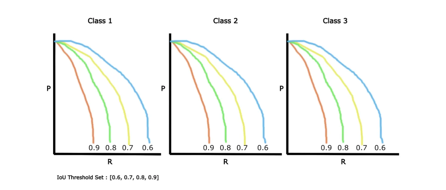
Data Scientists identified this weakness. They wanted the evaluation metric to be as robust as possible. So, they suggested measuring Average Precision for every class and every IoU threshold first and then calculating the average of the obtained scores.
Source
The picture above shows Precision-Recall curves drawn for 4 IoU thresholds for three different classes. In the example, the IoU threshold of 0.9 is the most stringent (as at least 90% overlap between the predicted and ground truth bounding boxes is required), and 0.6 is the most lenient.
As you can see, the difference between each IoU threshold value is 0.1. This measure is called a step. So, the abbreviation [email protected]:0.1:0.9 means that the mAP was calculated for each IoU threshold in the range [0.6, 0.7, 0.8, 0.9] and each class. Then the obtained values were averaged to get the final result.
Noteworthy, in the popular Common Objects in Context (COCO) dataset, mAP is benchmarked by averaging it out over IoUs from [0.5, 0.95] in 0.05 steps.
mean Average Precision calculation algorithm
Define the IoU thresholds;
Compute the Average Precision score for each IoU threshold for a specific class;
Calculate the mean Average Precision value for the given class by summing up the scores from step 2 and dividing them by the number of IoU threshold values;
Apply steps 2 and 3 to all the classes;
Sum up the obtained mAP scores and divide them by the total number of classes to get the final result.
What is Mask mean Average Precision?
To define the term, mask mean Average Precision (or mask mAP) is a variety of mean Average Precision. It is still a Machine Learning metric but designed to evaluate Instance Segmentation algorithms.
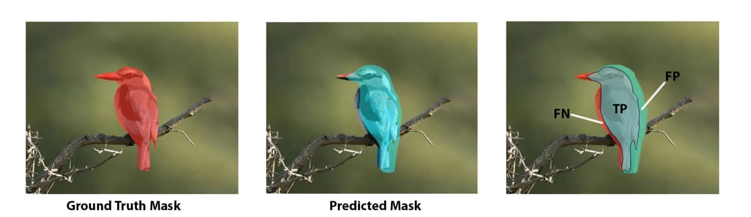
In short, mAP and mask mAP are similar when it comes to the calculation algorithm. The main difference is that IoU, in the mask mAP case, is calculated between segmentation masks instead of the bounding boxes. Beyond this, the mean Average Precision calculation algorithm is intact.
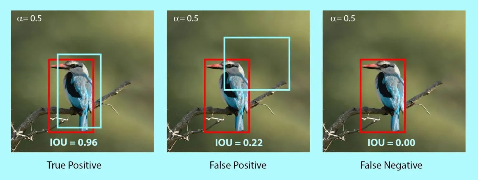
To visualize the difference, please take a look at the examples below. The first picture features an Object Detection task, as the ground truth labels are represented by bounding boxes. The second picture portrays an Instance Segmentation task, as the labels are pixel-perfect masks.
Source
Source
Interpreting mean Average Precision
Since mAP is calculated across multiple Precision-Recall curves, the best case scenario you can get is when both precision and recall metrics on every IoU threshold are equal to their best possible value – one. However, such a case is a fantasy, so you should stay realistic and expect a significantly lower metric value.
Noteworthy, it is complicated to provide unified mAP benchmarks that would suit any Object Detection problem since there are too many variables to consider, for instance:
the number of classes;
the expected tradeoff between Precision and Recall;
the IoU threshold, etc.
The truth is that based on the task, the same metric value might be both good and bad. So, if you spend some time identifying the desired value for your case and estimating your goals and resources, it would benefit you greatly.
Nevertheless, the SOTA (State-of-the-Art) mAP for the Object Detection task on the COCO dataset's test part is currently 63,1.
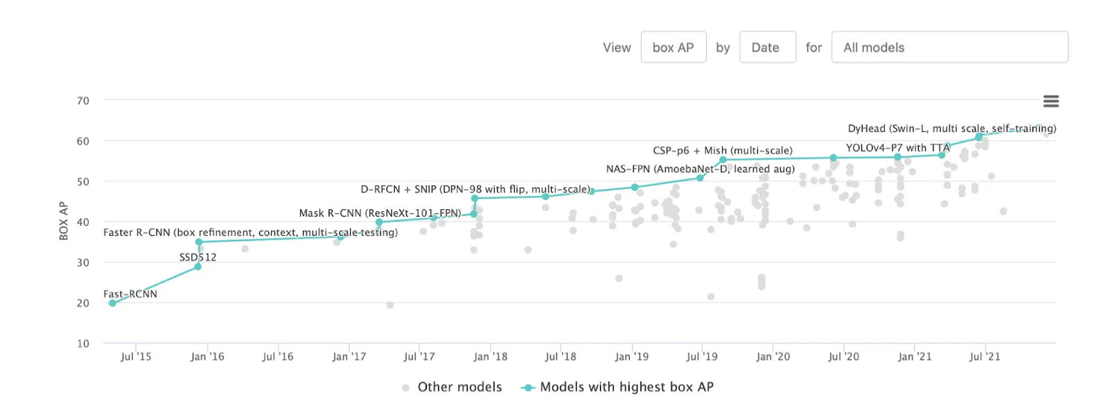
Source
As you can see, SOTA is relatively low. Still, it does not mean you should stop if you see a value similar to it in your task. From our experience and the research conducted when writing this page, if your task does not include millions of classes and your IoU threshold is set to 0,5, you should reach at least 0,7 mAP before you are more or less satisfied with the model's performance.
To summarize, if your Object Detection task is not similar to COCO, you should not bother that much about SOTA and try to achieve 0,8 mAP on the 0,5 IoU threshold before calling the job done. Also, do not trust the metric alone and always visualize the model's predictions to ensure your solution works as intended.
mean Average Precision calculation example
For this page, we decided to be more advanced and prepared a Google Colab notebook featuring calculating mAP using Python on a simple example. We used the Average Precision and mean Average Precision formal formulas, NumPy and Sklearn functionalities, and some imagination.
If you want a well-commented yet simple example of computing mean Average Precision in Python, check out this example.
mean Average Precision in Python
The mean Average Precision score is widely used in the industry, so the Machine and Deep Learning libraries either have their implementation of this metric or can be used to code it quickly. For this page, we prepared three code blocks featuring calculating mAP in Python. In detail, you can check out:
mean Average Precision in NumPy;
mean Average Precision in TensorFlow;
mean Average Precision in PyTorch.