
The EU AI Act mandates human oversight for ethical AI. CloudFactory's human-in-the-loop solutions ensure accuracy, security, and compliance.
CloudFactory Blog
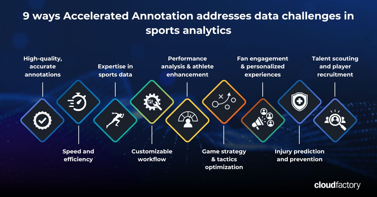
Say goodbye to data challenges. Learn how investing in high-quality data labeling fuels winning ML models in sports analytics.
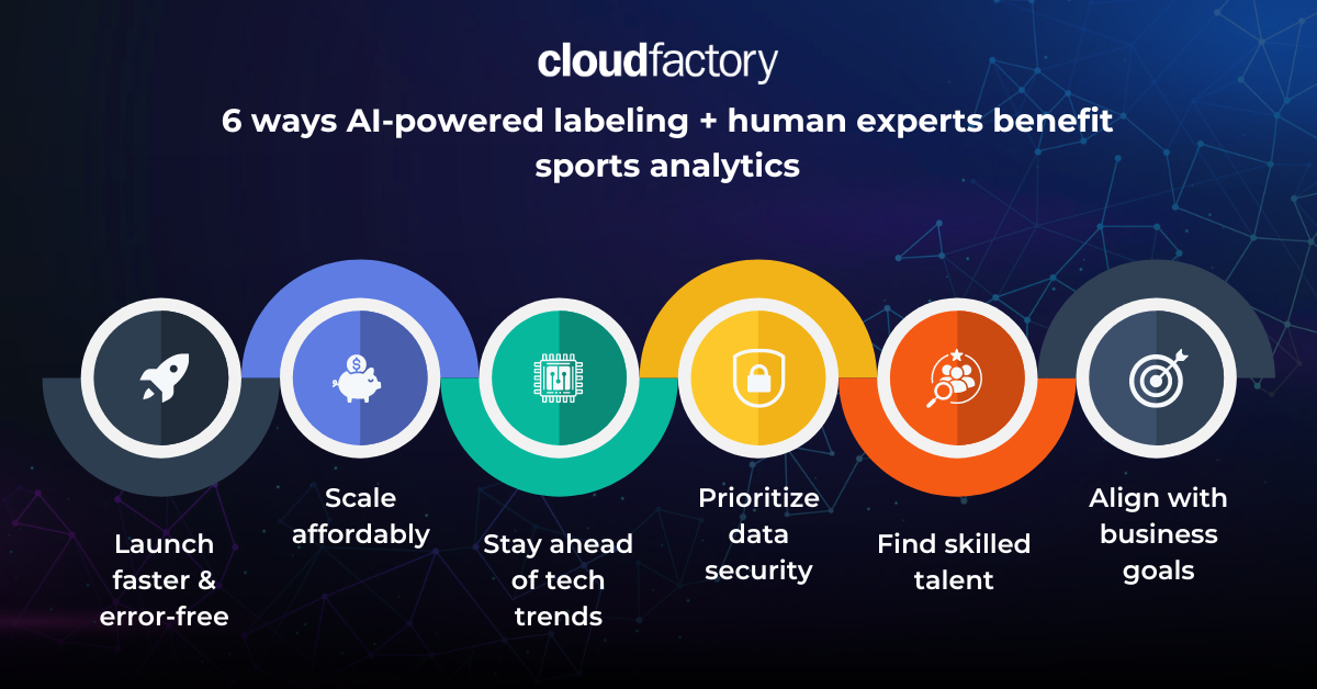
The key to faster ROI, lower costs, and new revenue streams in sports analytics is integrating AI-powered data labeling and human expertise.

Expert strategies for eliminating data bottlenecks, scaling your ML data labeling pipeline, optimizing your workforce, and unlocking faster AI insights.

Discover the impact of quality data labeling in infrastructure asset management. Learn ML model accuracy, performance, and scalability strategies in asset inspection and ...

Find the right ML data labeling tools for your business in 2024. Optimize process, maximize data quality, and boost ROI with expert guidance.

Learn 5 practical strategies to avoid AI disappointment and achieve success using a combination of technology and human expertise.
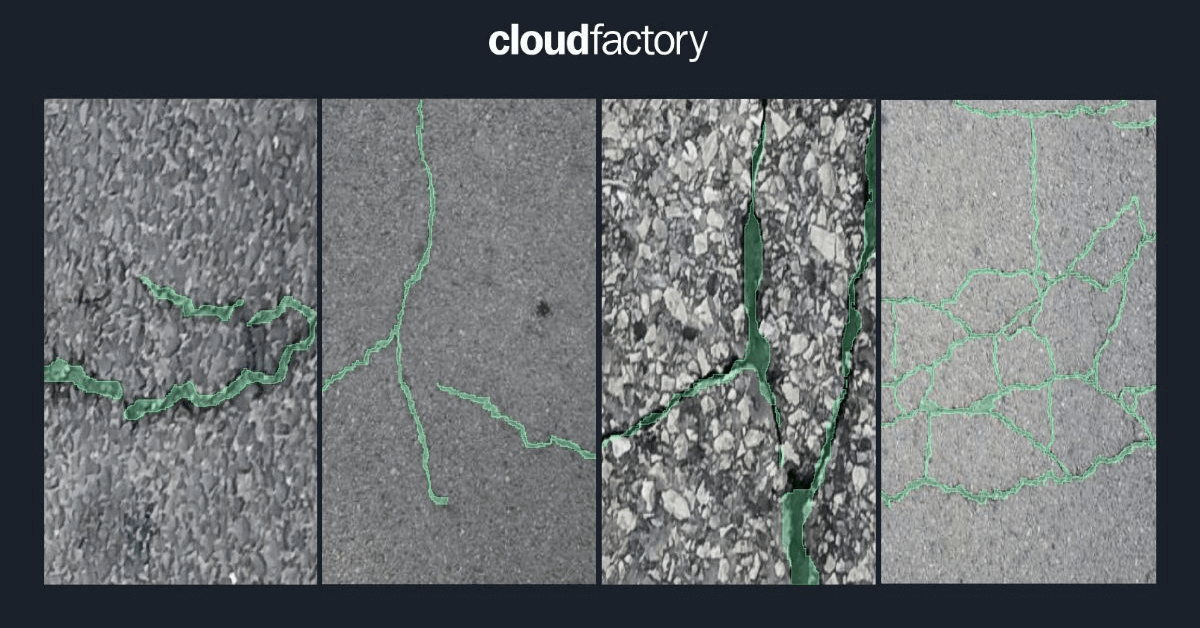
Discover the impact of quality data labeling in infrastructure asset management. Learn ML model accuracy, performance, and scalability strategies in asset inspection and crack ...

Quality data labeling fuels infrastructure health. Learn how to achieve ML model accuracy, performance, & scalability to extend asset life.

LiDAR is a useful 3-D object detection technology for many industries, from AV to aerial inspections. Here are 7 interesting applications of LiDAR.

How CTOs and VPs of product and machine learning can navigate key agtech hurdles using AI-powered data labeling for sustainable growth and profitability.

While foundational models offer remarkable potential, our experience reveals that humans in the loop remain crucial for successful AI development.

Discover the impact of quality data labeling in agtech. Learn ML model accuracy, performance, and scalability strategies in precision farming.

Happy Birthday, Accelerated Annotation! It's been a year of providing clients with the quality training data needed to launch your models fast.

Learn the four workforce traits crucial for high-quality ML datasets. Avoid costly rework and boost your AI project's success.

This post discusses image segmentation challenges developers face across the ML pipeline - from data annotation to the deployment stage of the lifecycle.
